karsttech.com/content/professional-projects/usm-magnetics-machine-learning/index.md

+++ title = 'Machine Learning for Magnetic Target Detection' description = 'Using machine learning to detect and localize magnetic targets underwater' date = 2025-04-03T16:00:00-05:00 draft = false categories = ['USM', 'magnetics'] tags = ['data science', 'KarstTech', 'UUV', 'modeling', 'machine learning', 'AI'] +++

Using machine learning to detect and localize magnetic targets underwater

{{< katex >}}

Machine Learning for Target Classification and Localization

I wanted to share some exciting progress from our recent efforts to detect, classify, and localize magnetic targets underwater. So today we're diving deeper into machine learning approaches.

Magnetic Modeling Foundation

We've established three distinct magnetic modeling techniques, each with different advantages:

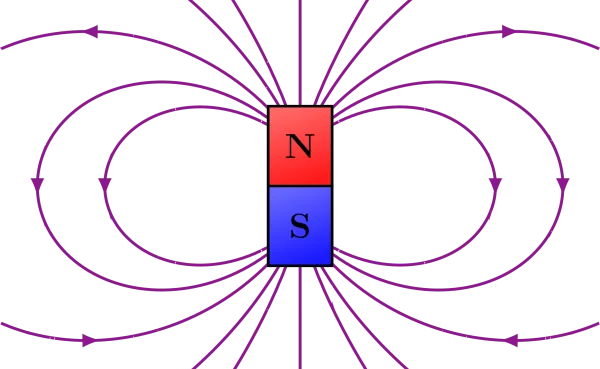
1. Simple Dipole Model - This is the most basic type of magnetic model, and so also the fastest to calculate, making it ideal for generating billions of examples for initial AI training. We rely on magpylib to calculate the magnetic field near a dipole source as it provides a simple API for the underlying numpy array calculations. The parameters of the dipole are provided based on an expected range of target properties. The equation for the magnetic field of a dipole is given by:

\vec{B}(\vec{r}) = \frac{\mu_0}{4\pi} \left[ \frac{3\vec{r}(\vec{m} \cdot \vec{r})}{r^5} - \frac{\vec{m}}{r^3} \right]

• \( \vec{B} \) is the magnetic field vector
• \( \vec{r} \) is the position vector of the field point
• \( \vec{m} \) is the magnetic dipole moment vector
• \( \mu_0 \) is the permeability of free space
• \( \pi \) is the mathematical constant pi

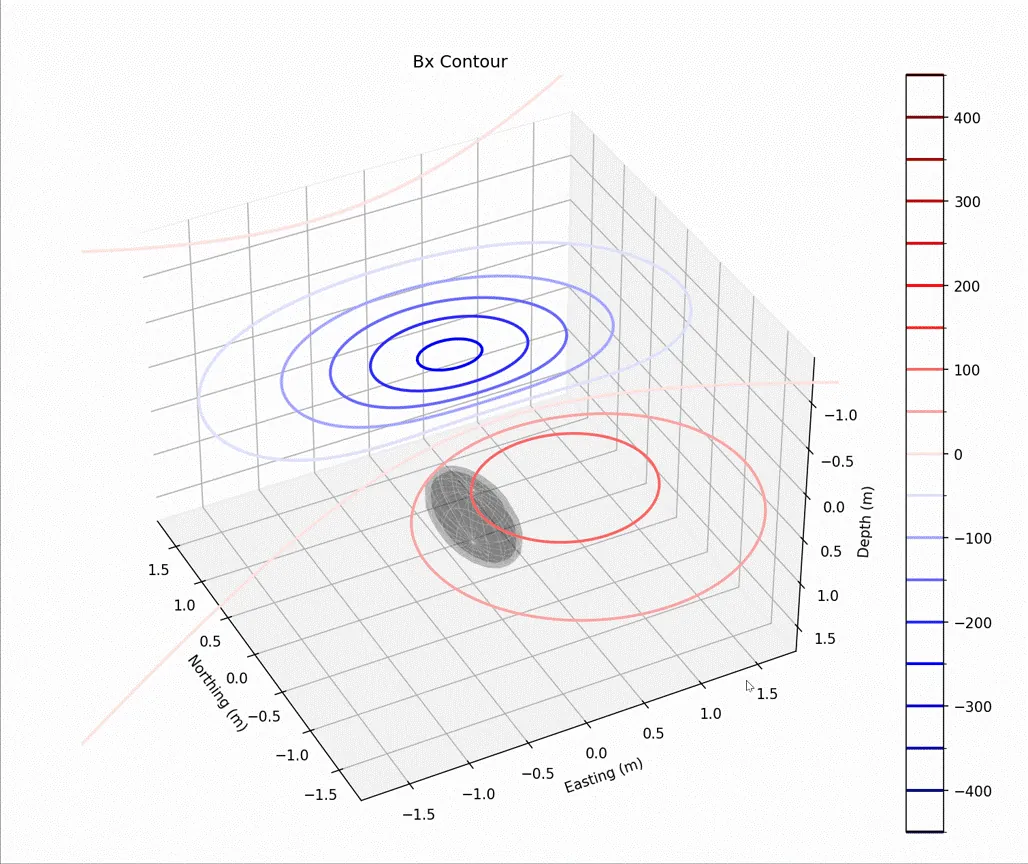
2. Ellipsoid Modeling - Developed in partnership with Colorado School of Mines, this technique efficiently models triaxial ellipsoids with full support for magnetic induction and self-demagnetization effects. These models are perfect for AI training since they can generate realistic data on-the-fly. Ellipsoids are the most complex geometry for which we have a closed-form solution for the magnetic field including self-demagnetization, and so it is the most complex type of target for which we can generate individual sensor samples without needing to simulate the entire target and environment. More complex geometries can be estimated by using multiple ellipsoids and adding or subtracting them from each other. This method is imperfect because the induction and demagnetization effects between ellipsoids are not taken into account.

The mathematical model for these ellipsoids is too complex to describe here, but our techniques are based on this paper: Ellipsoids (v1.0): 3-D magnetic modelling of ellipsoidal bodies

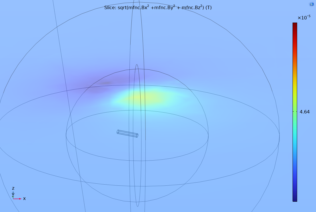
3. COMSOL Multiphysics Simulation - Our most accurate modeling technique that fully supports magnetic induction and self-demagnetization with arbitrary target geometries. These models have been validated against real-world test data, but are computationally expensive to run.

ML Progress

{{< mermaid >}} flowchart TD subgraph "Example CNN Architecture" A["Position Input [N, 3]"] --> C B["Magnetometer Input [N, 3]"] --> C C["Conv2D: 3→64"] --> D D["Conv2D: 64→128"] --> G

E["Mag DC Offsets [3]"] --> I
F["Position / Mag Scaling Factors [2]"] --> I

G["Conv2D: 128→256"] --> H
H["Global AvgPool"] --> K

I["Linear: 5→32"] --> J
J["Linear: 32→32"] --> K

K["Feature Concat"] --> L
L["Dense Layers"] --> M
M["Output Layer"]
end

{{< /mermaid >}}

Building on this foundation for magnetic target modeling, we have created a series of machine learning models which have proven able to predict target location, orientation, and magnetic strength with impressive accuracy despite their low parameter count.

Beginnings

Our initial models were scattered attempts to see which general types of neural networks would work best for this task. LSTM, RNN, and CNN models were all tried, and none performed very well for various reasons. Eventually a hybrid approach was found to preprocess the magnetic data to normalize it, and then use a CNN to learn the features within the normalized data. The extracted scaling factors and DC offsets were then used to feed into the deeper layers of the network to give the model information about field strength. This was primarily done to combat a vanishing gradient problem that occurs when target strengths vary by many orders of magnitude, both due to the variance in expected target strengths, and also due to the fact that the magnetic field strength of a dipole falls off as the cube of the distance from the target, and our distances to target vary significantly.

These hybrid CNN models were explored using parameter sweeps to optimize their geometry, and the results for target localization were nearly perfect to within the expected error introduced as noise in the input data. Target orientation and magnetic strength were also predicted, but with poor accuracy.

Improvements

Several methods were explored to improve the accuracy of the model, including:

• Changing the loss functions to prevent vanishing gradients followed by NaN propagation.
• Attention mechanisms within the model were explored, but these also showed no improvement.
• Changing the orientation representation within the training data / model output to be more consistent and easier to learn.
  • Euler angles were used at first, but these had many problems.
  • Quaternions were tried in an attempt to address uniformity and gimbal lock issues, but with little to no improvement.
  • Gram-Schmidt orthogonalization was used to ensure that the orientation vectors were orthogonal, and that the gradient was smooth for all changes in angle. This was expected to solve the problem, but showed minimal advantage over the other methods.
  • The most successful method found was to encode the orientation and the magnetic strength into a single 3-vector, rather than encoding them separately. This representation is presumed to be successful because the vector representation of magnitude allows for more linear relationships between the model output and the input, which are more easily modeled and learned by the network.

3D Convolutional Layers

In addition to the loss function changes and orientation representation iterations, one of the most significant improvements was switching from 2D to 3D convolutional layers in our neural networks. This allows the model to better understand the relationships between sensor positions and vector field components, dramatically improving performance per parameter count. The three dimensions of the input data in question are Sample Number, Sensor Position (X,Y,Z), and Vector Field Component (X,Y,Z).

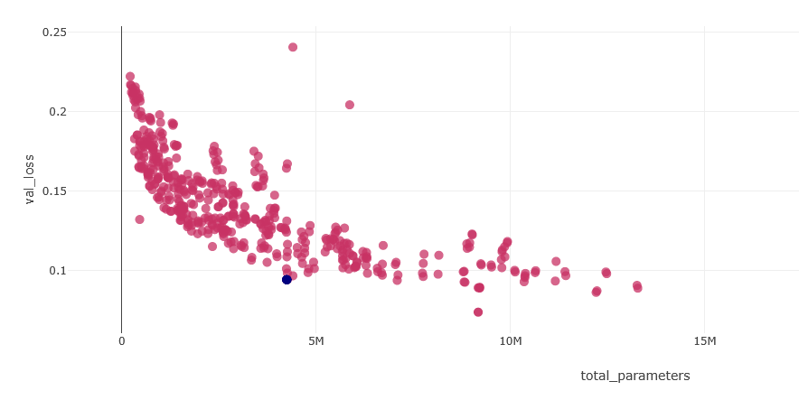
Though Loss in this context is somewhat loosely defined without looking at the loss equations, the performance of the model was improved by several times over, corresponding to a reduction in loss by a factor of 1/2 or better for equivalent parameter counts and training times. The blue dot in the plot below shows the performance of the best model which includes all of the improvements mentioned above, and red dots show other configurations which were explored, with the far upper right two dots showing the initial models. Note that the initial and final model architectures are not directly comparable due to changes to their loss functions, though it is expected that this would make the improvements even more pronounced.

Model Performance Stats

The current best model seems to be performing quite well!

• 99.72% of predictions are within 1m or 20% of actual target position
• 97.24% of predictions are within 0.3m or 10% of actual target position
• The model works for targets between 3-15m from closest approach
• ~4.5M parameters, which can easily run on low power hardware onboard the UUV
• Inference time is extremely fast (0.02ms on an RTX 4090), meaning it should run well under one second on the actual UUV hardware

The cases where the model gives poor predictions seem to be primarily when the simulated target is very weak and the point of closest approach is at a large distance, which is expected. No attempt is made while creating input data to validate that a given target is detectable under the noise floor, and so this issue is expected.

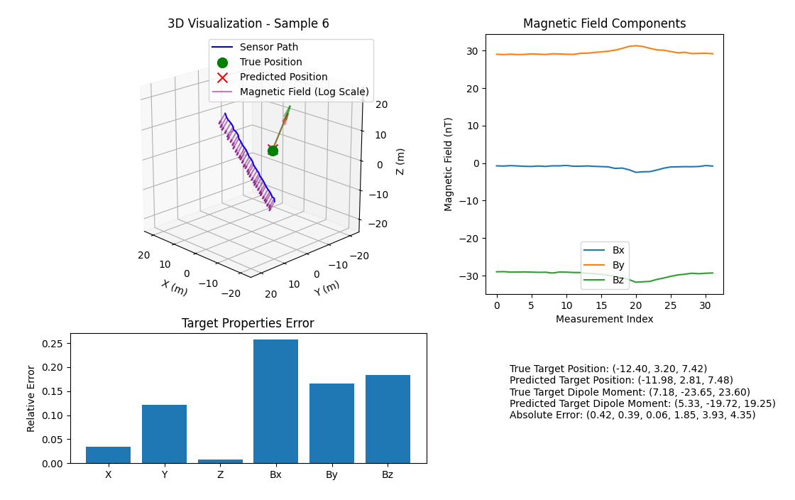
The visualization above shows the chosen model target prediction capability for one example in the validation data set. The model never saw this data point during training, and its location prediction is within approximately 0.35m from a closest approach of 9.61m. The target orientation prediction is accurate to within 1.335 degrees despite the magnetic moment from which it is derived containing a high ~30% error. This high magnetic moment error is in part due to the added noise combined with the high sensitivity of the predicted moment magnitude to errors due to the inverse cubed falloff nature of magnetic fields. Prediction accuracy, and especially magnetic moment prediction accuracy improves at closer ranges and larger magnitude targets.

Parametric Inversion Method

In addition to machine learning, we developed a first principles approach using parametric inversion. This technique:

• Constructs a mathematical model of the relationship between magnetic sources and observable fields
• Uses optimization to solve the inverse problem and recover target properties
• Provides well-defined behavior that can serve as a benchmark for ML solutions
• Is limited only by input data quality and can provide high precision with good measurements

While not as noise-tolerant as our ML approach, the parametric inversion method offers reliable, physics-based results without the risk of unexpected behavior in novel conditions. I might write more about this in a future post since it deserves a more detailed explanation.

Next Steps

For our next phase, we'll be focusing on:

• Expanding our ML models to handle complex magnetic signatures from multiple targets
• Integrating formal classification frameworks with our extracted parameters
• Testing with real-world data from our UUV platform
• Optimizing for embedded systems with limited hardware resources

The ultimate goal remains enhancing UUV capabilities for detecting underwater objects, and using magnetic sensing to complement traditional navigation methods.

I'm excited to see how these models perform in upcoming open water tests with real UUVs in the near future!