6.3 KiB
+++ title = 'USM Magnetics - Magnetic Parametric Inversion' date = 2025-04-04T14:00:00-05:00 draft = false categories = ['USM', 'magnetics'] tags = ['data science', 'KarstTech', 'modeling'] +++
{{< katex >}}
Magnetic Dipole Localization: Methods for Parametric Inversion
In the previously discussed ML based methods for magnetic target localization, we trained and tested models from simulated data. In the case that we are working with near perfect data, the problem that the ML models approximate is the same as the method of parametric inversion. If well trained, the hope is that the ML models will perform better than parametric inversion in the real world, but developing the inversion method provides a good baseline for comparison, both for computational complexity and for accuracy.
So what is Parametric Inversion?
Parametric inversion is a method for estimating the position and magnetic moment of a magnetic dipole from the field it creates. It is a physics-based method that is relatively simple to understand and implement, and is therefore a good baseline for comparison to the ML based methods. In essence, we set up a system of equations that describes the magnetic field at a given set of measured points in space due to the dipole and it's properties, then we solve this overdetermined system of equations using optimization.
The magnetic field of a dipole at position \( \vec{r} \) relative to the dipole is given by:
\vec{B}(\vec{r}) = \frac{\mu_0}{4\pi} \frac{3(\vec{m} \cdot \hat{r})\hat{r} - \vec{m}}{|\vec{r}|^3}
Expanding this out in cartesian coordinates, we get:
% Expanded form with vector components
\begin{pmatrix} B_x \ B_y \ B_z \end{pmatrix} = \frac{\mu_0}{4\pi} \frac{1}{r^3} \left[ 3 \frac{(m_x r_x + m_y r_y + m_z r_z)}{r^2} \begin{pmatrix} r_x \ r_y \ r_z \end{pmatrix} - \begin{pmatrix} m_x \ m_y \ m_z \end{pmatrix} \right]
Where:
- \( (x_0, y_0, z_0) \) represents the coordinates of the dipole's position
- \( (x_i, y_i, z_i) \) represents the coordinates of the $i$-th measurement point
- \( (r_x, r_y, r_z) \) or \( \vec{r}_i \) represents the vector from the dipole to the measurement point
- \( (m_x, m_y, m_z) \) are the components of the dipole moment vector
- \( (B_{x}, B_{y}, B_{z}) \) or \( \vec{B} \) are the measured field components at a point
- \( \mu_0 \) is the magnetic permeability of free space
Once we set up the system of equations, we can optimize for the least squares solution for the dipole moment and position vectors \( \vec{m} \) and \( \vec{r} \). In my case, I used the scipy.optimize.least_squares function to do this, but this may soon be replaced by a custom simulated annealing approach. One other place where this may be improved is weighting the uncertainty in measurements according to the distance from the dipole, as the field strength is inversely proportional to the cube of the distance, and lower strength measurements are more prone to error from noise.
Data Preparation
Before we can use a solver for the parametric inversion, it can be useful to estimate the dipole properties using some other methods. This can help ensure the optimizer converges to the correct solution, and does not get stuck in a local minimum, or use more than the necessary computational resources.
Background Field Estimation
In our simulations, we have more than just the field from the dipole to contend with. We have the background field from the Earth, and we have other fields from noise sources like the UUV itself. The approach begins by distinguishing the dipole field from background fields (like Earth's magnetic field). It identifies regions where field variations are minimal and consistent, suggesting background dominance rather than dipole influence. This is done by:
- Analyzing field derivatives to find areas of low variation
- Evaluating local field consistency within sliding windows
- Combining these metrics to identify the most reliable background-dominated regions
Position Estimation
The dipole's position is estimated through analysis of the field pattern along the measurement line. The method uses several key insights:
- The maximum field strength typically occurs at the point nearest to the dipole
- The Full Width at Half Maximum (FWHM) of the field magnitude profile relates to the perpendicular distance to the dipole (roughly FWHM ≈ 2h, where h is the distance)
- This initial estimate is then refined using pattern-matching optimization
The physics behind this relies on the rapid decay of dipole fields with distance (proportional to 1/r³), which creates distinctive spatial patterns.
Dipole Moment Calculation
Once the position is established, the dipole's magnetic moment is calculated as described above. These equations are used to construct a system of linear equations for all measurement points, which is then solved using regularized least squares to find the dipole moment vector.
Orientation Analysis
From the moment vector, the dipole's orientation is characterized by:
- Magnitude (strength of the dipole)
- Polar angle θ (angle from the vertical) \( \theta = \arccos\left(\frac{m_z}{|\vec{m}|}\right) \)
- Azimuthal angle φ (angle in the horizontal plane) \( \phi = \arctan2(m_y, m_x) \)
Results
The quality of the inversion is typically quite good. The example below has included jitter in the measurement path, as well as 2% noise in the field measurements.
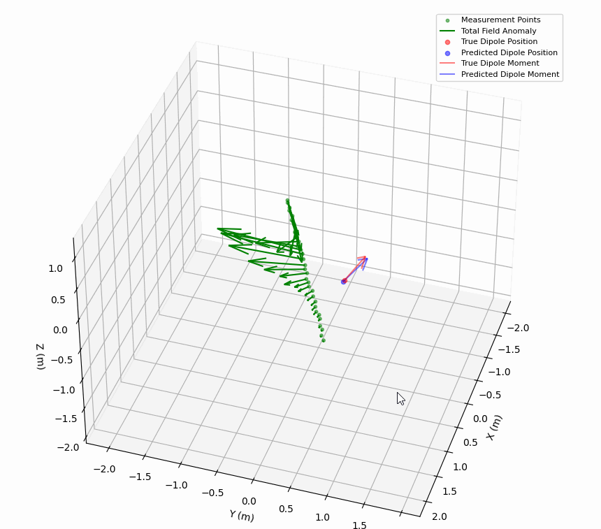
Position:
True:      -7.00e-01, +3.00e-01, -1.00e+00
Predicted: -6.90e-01, +2.80e-01, -1.02e+00

Dipole moment:
True:      +1.00e-05, +1.00e-05, +2.00e-05
Predicted: +9.65e-06, +1.12e-05, +1.99e-05

Dipole orientation angles:
  True θ (polar):      35.3°
  Predicted θ (polar): 36.6°
  True φ (azimuthal):      45.0°
  Predicted φ (azimuthal): 49.2°

Relative error:
  Field: 2.50%
  Position: 4.09%
  Moment: 4.98%
This approach produces a comprehensive characterization of a magnetic dipole, including its position and moment vector with implied orientation angles, along with error metrics to assess the quality of the inversion. This will be used both as a benchmark for ML approaches, and possibly as an alternative to ML approaches for real-time or resource limited applications. The implementation is being actively developed, but I might share it here in the future.